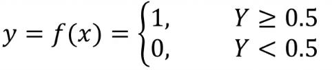
机器学习中采用逻辑回归算法解决分类问题 在忙碌的工作中,还是需要抽时间来记录一下学习所得,在上一篇文章中我们谈到了使用线性回归来预测房价的问题,在这篇文章中我们谈一谈逻辑回归。
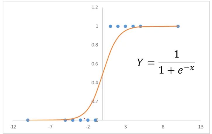
我对逻辑回归的理解 这几天学了一下逻辑回归,总的来说,我认为主要还是用来解决分类问题中的二分类(其实还可以做多分类,但是不是主要),多分类的话可以采用之后所说的非监督学习。在上一篇文章中,我们在线性回归算法中对模型的评估主要是用MSE,R2_score这两种损失函数的方法,而在逻辑回归算法中,我们使用准确率来对模型进行评估。
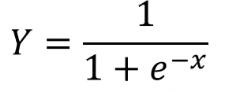
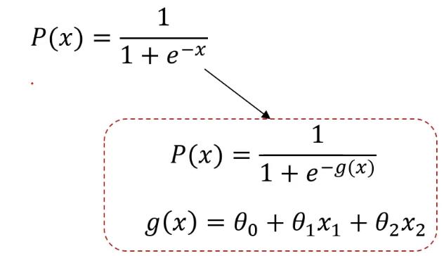
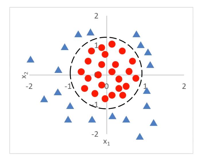
关于逻辑回归方程 sigmoid函数也叫Logistic函数,用于隐层神经元输出,取值范围为(0,1),它可以将一个实数映射到(0,1)的区间,可以用来做二分类。在特征相差比较复杂或是相差不是特别大时效果比较好。Sigmoid作为激活函数有以下优缺点:
当问题更复杂时,可以用g(x)代替x,然后就可以根据g(x)寻找最合适的决策边界从而解决二分类问题。
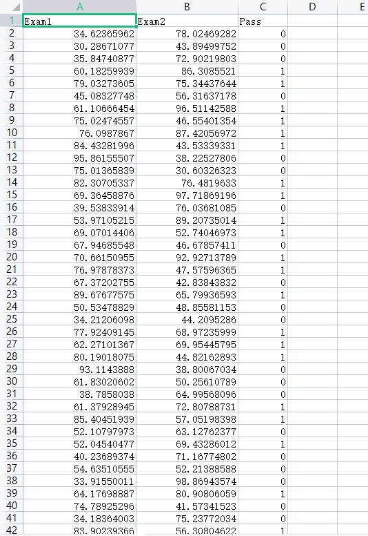
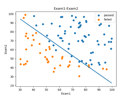
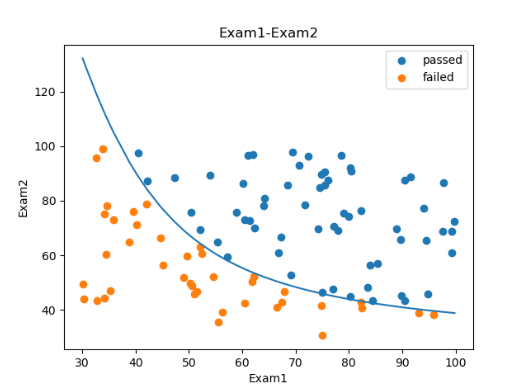
使用逻辑回归算法对考试成绩进行预测 基于examdata.csv数据,建立逻辑回归模型 预测Exam1 = 70, Exam2 = 60时,该同学在Exam3是 passed or failed; 建立二阶边界,提高模型准确度。
⭐预测数据展示
⭐代码展示
1
2
3
4
5
6
7
8
9
10
11
12
13
14
15
16
17
18
19
20
21
22
23
24
25
26
27
28
29
30
31
32
33
34
35
36
37
38
39
40
41
42
43
44
45
46
47
48
49
50
51
52
53
54
55
56
57
58
59
60
61
62
63
64
65
66
67
68
69
70
import numpy as npimport pandas as pdfrom matplotlib import pyplot as pltfrom sklearn.linear_model import LogisticRegressionfrom sklearn.metrics import accuracy_scoredata = pd.read_csv('examdata.csv' ) mask = data.loc[:,'Pass' ]==1 X = data.drop(['Pass' ],axis=1 ) y = data.loc[:,'Pass' ] X1 = data.loc[:,'Exam1' ] X2 = data.loc[:,'Exam2' ] X1_X1 = X1*X1 X1_X2 = X1*X2 X2_X2 = X2*X2 LR = LogisticRegression() LR.fit(X,y) theta0 = LR.intercept_ theta1 = LR.coef_[0 ][0 ] theta2 = LR.coef_[0 ][1 ] predict_y = LR.predict(X) result = accuracy_score(y,predict_y) print (data.head())fig = plt.figure() passed = plt.scatter(X1[mask],X2[mask]) failed = plt.scatter(X1[~mask],X2[~mask]) plt.xlabel('Exam1' ) plt.ylabel('Exam2' ) plt.title('Exam1-Exam2' ) plt.legend((passed,failed),('passed' ,'failed' )) X2_new = -(theta0+theta1*X1)/theta2 plt.plot(X1,X2_new) plt.show()
⭐一阶边界结果
⭐二阶边界结果
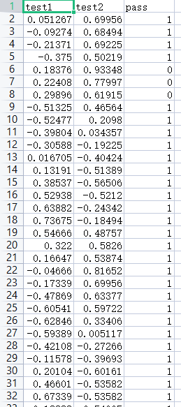
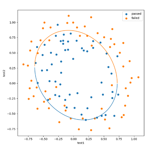
使用逻辑回归算法对芯片进行检测 ⭐思路与过程
⭐预测数据展示
⭐代码展示
1
2
3
4
5
6
7
8
9
10
11
12
13
14
15
16
17
18
19
20
21
22
23
24
25
26
27
28
29
30
31
32
33
34
35
36
37
38
39
40
41
42
43
44
45
46
47
48
49
50
51
52
53
54
55
56
57
58
59
60
61
62
import numpy as npimport pandas as pdfrom matplotlib import pyplot as pltfrom sklearn.linear_model import LogisticRegressionfrom sklearn.metrics import accuracy_scoredata = pd.read_csv('chip_test.csv' ) x = data.drop(['pass' ],axis=1 ) y = data.loc[:,'pass' ] x1 = data.loc[:,'test1' ] x2 = data.loc[:,'test2' ] mask = data.loc[:,'pass' ]==1 LR1 = LogisticRegression() LR1.fit(x,y) y_predict = LR1.predict(x) print (accuracy_score(y, y_predict)) x1_2 = x1*x1 x2_2 = x2*x2 x1_x2 =x1*x2 x_new = {'x1' :x1,'x2' :x2,'x1_2' :x1_2,'x2_2' :x2_2,'x1_x2' :x1_x2} x_new = pd.DataFrame(x_new) LR2 = LogisticRegression() LR2.fit(x_new,y) y_predict = LR2.predict(x_new) print (accuracy_score(y, y_predict))x1_new = x1.sort_values() theta0 = LR2.intercept_ theta1 = LR2.coef_[0 ][0 ] theta2 = LR2.coef_[0 ][1 ] theta3 = LR2.coef_[0 ][2 ] theta4 = LR2.coef_[0 ][3 ] theta5 = LR2.coef_[0 ][4 ] def f (x1_new ): a = theta4 b = theta2+theta5*x1_new c = theta0+theta1*x1_new+theta3*x1_new*x1_new x2_new_boundary1 = (-b+(np.sqrt(b*b-4 *a*c)))/(2 *a) x2_new_boundary2 = (-b-(np.sqrt(b*b-4 *a*c)))/(2 *a) return x2_new_boundary1,x2_new_boundary2 x1_range = [-0.9 + x/10000 for x in range (0 ,19000 )] x1_range = np.array(x1_range) x2_new_boundary1 = [] x2_new_boundary2 = [] for x in x1_range: x2_new_boundary1.append(f(x)[0 ]) x2_new_boundary2.append(f(x)[1 ]) fig1 = plt.figure() plt.figure(figsize=(8 ,8 )) passed = plt.scatter(x1[mask],x2[mask]) failed = plt.scatter(x1[~mask],x2[~mask]) plt.xlabel('test1' ) plt.ylabel('test2' ) plt.legend((passed,failed),('passed' ,'failed' )) plt.plot(x1_range,x2_new_boundary1) plt.plot(x1_range,x2_new_boundary2) plt.show()
⭐二阶边界结果